Atomic Term Symbols: Part 2 - Term Symbols and Spin-Orbit Coupling

Introduction

This article is an in-depth explanation on atomic term symbols based on Quantum Chemistry by Levine to supplement chapter 8 of Physical Chemistry: A Molecular Approach by McQuarrie. A good understanding of preceding chapters, notably chapters 6 and 7, is required.

The notation used in this article is based on the latter textbook.

In Part 1, we looked at how quantum numbers can describe an atomic energy state. In this article, we will see how term symbols can describe an energy level. In Part 3, we will go over more complex examples of term symbols, as well as Hund’s Rules.

Energy State and Energy Level

In physical chemistry and quantum mechanics, we talk a lot about energy states and energy level - oftentimes interchangably. However, a clear distinction should be made between the two in order to clear up confusion.

An energy state is a wave function with a definite energy. It satisfies the time-independent Schrödinger equation $\hat{H}\psi = E\psi$. They are also called stationary states due to the fact that the wave function does not change with time (apart from its phase).

An energy level is a value of energy that a system can have. It can consist of a single energy state or many, with the latter case being regarded as degenerate.

Why Electron Configuration ≠ Energy State Nor Level

In general chemistry, two representations of electron configurations are taught, as shown below for ground-state carbon.

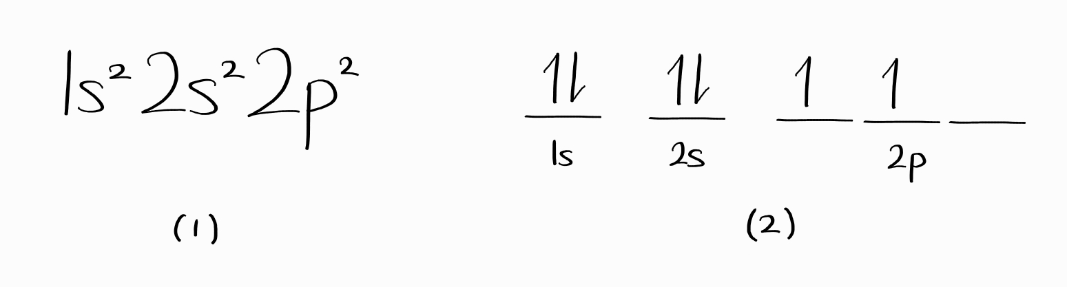
It is frequently understood that the two forms, (1) and (2), indicate the energy state or the energy level. That is incorrect.

For (1), many energy states (wave functions) have this electron configuration. Even worse, these states from a single electron configuration can correspond to several different energy levels.

The diagram (2) is misleading as $\psi$ constructed exactly in this way would not follow the Pauli antisymmetry principle. In fact, you would need to have a linear combination of such $\psi$ to obtain proper energy state. As a result, an overwhelming number of such diagram has to be used to express a single energy level.

It is clear that either electron configurations ((1) and (2)) are inadequate at expressing either energy state or energy level. On the other hand, we ended Part 1 with a way to express an energy state, in the form of

$$\psi = \left |\, (e^- \text{ config)}\,L\,M_L\,S\,M_S\,\right \rangle$$

In Part 2, we introduce atomic term symbols, which is a convenient way to express an energy level of an atom.

Atomic Term Symbols

Before we begin, we need to know what determines the energy of an energy state $\left |\, (e^- \text{ config)}\,L\,M_L\,S\,M_S\,\right \rangle$. First, the electron configuration is the biggest factor in determining the energy. Second, $S$ also affects the energy; recall Hund’s rule from general chemistry where the lowest energy electron configuration is the one with the most parallel spins. At last, $L$ affects the energy, albeit to a lesser degree than the two aforementioned factors. This is closely related to how the orbital energy of multi-electron atoms are determined in part by $l$ ($s < p < d < f < \cdots$), unlike hydrogen-like atoms ($s = p = d = f = \cdots$).

$M_L$ and $M_S$ do not have any effect on the energy. In other words, energy states with (1) the same electron configuration, (2) the same $L$, and (3) the same $S$ are degenerate. This leads to an interesting conclusion:

The energy level of an atom is determined by the electron configuration, the total orbital angular momentum quantum number $L$, and the total spin quantum number $S$.

To express the energy level of an atom, we introduce atomic term symbols,¹ which express $L$ and $S$ in the following form.

$$^{2S+1}L$$

Instead of substituting $L$ with a number, we use letters similar to that of atomic orbitals:

$L \,=$	0	1	2	3	4	5	$\cdots$
	$S$	$P$	$D$	$F$	$G$	$H$	$\cdots$

Instead of $S$, we denote the spin multiplicity, which is equal to $2S+1$. As $M_S = -S, \,-S+1,\, \cdots ,\,+S-1,\,+S$, $2S+1$ is in fact the total number of $M_S$ and is the degeneracy due to spin. Keep in mind that $M_L = -L, \,-L+1,\, \cdots ,\,+L-1,\,+L$, and that a total of $2L+1$ different $M_L$ are possible for a particular value of $L$. Thus, $2L+1$ is the degeneracy due to orbital angular momentum.

Therefore,

The degeneracy of an energy level of an atom is equal to $\left(2L+1\right)\left(2S+1\right)$

Let us work on some example to understand term symbols. The ground level of hydrogen is expressed as $1s^1 : ^2S$. This means that $S = 1/2$ (as $2S+1 = 2$) and $L = 0$. Energy states for this ground level can have $M_L = 0$ and $M_S = +1/2, -1/2$. Therefore, in bra-ket notation, the energy states $\left |\, 1s^1\,0\,0\,\frac{1}{2}\,+\frac{1}{2}\,\right \rangle$ and $\left |\, 1s^1\,0\,0\,\frac{1}{2}\,-\frac{1}{2}\,\right \rangle$ both have the same energy level $1s^1 : ^2S$. This energy level has a degeneracy of 2, which can be obtained by inspection, and also by multiplying the spin multiplicity $2S+1$ by $2L+1$.

Note that the term symbol $^2S$ is read “doublet $S$”, owing to its spin multiplicity. Here are names for other spin multiplicities.

$S$	Spin Multiplicity: $2S+1$	Name
$0$	$1$	Singlet
$\frac{1}{2}$	$2$	Doublet
$1$	$3$	Triplet
$\frac{3}{2}$	$4$	Quartet
$2$	$5$	Quintet
$\frac{5}{2}$	$6$	Sextet

A more complicated example is ground level nitrogen with $1s^22s^22p^3 : ^3P$ (read as “triplet $P$”). From the term symbol, $L=1$ and $S=1$. The degeneracy of this energy level is $(2\times1+1)(2\times1+1) = 9$. All nine energy states are ground states of nitrogen.

The Value of $L$ and $S$: $1s^1 2s^1$

Say you want to know the term symbols associated with an excited helium atom with an electron configuration of $1s^1 2s^1$. The easiest way to obtain the term symbols (i.e. energy levels) would be to first identify all wave functions (i.e. energy states). In the process of identifying all energy states $\left |\, (e^- \text{ config)}\,L\,M_L\,S\,M_S\,\right \rangle$, the $L$ and $S$ required for the term symbol are automatically revealed.

Therefore, we first construct the wave functions (more precisely, spin orbitals) of $1s^1 2s^1$.

Approach 1: the naive approach

One thing to note about electronic wave functions is that they are antisymmetric: the exchange of two electrons results in the same wave function with the opposite sign. With this in mind, let us start by naïvely constructing wave functions from electron configurations, also called microstates².

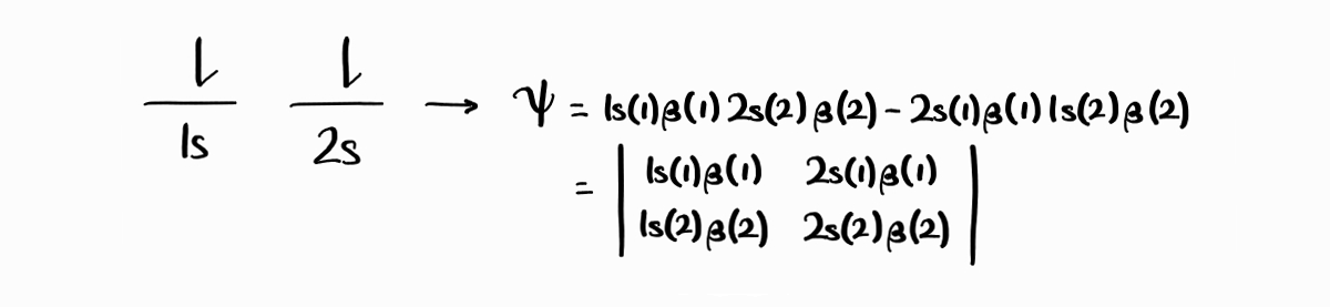
A plausible wave function for the first microstate, with both electrons spin up, is $1s(1)\alpha(1)\,2s(2)\alpha(2)$ (this means electron 1 is in $1s$ with spin up, electron 2 is in $2s$ with spin up).³ Due to the indistinguishability of electrons, the $2s$ electron can be electron 1 as well. This results in another potential wave function: $2s(1)\alpha(1)\,1s(2)\alpha(2)$.

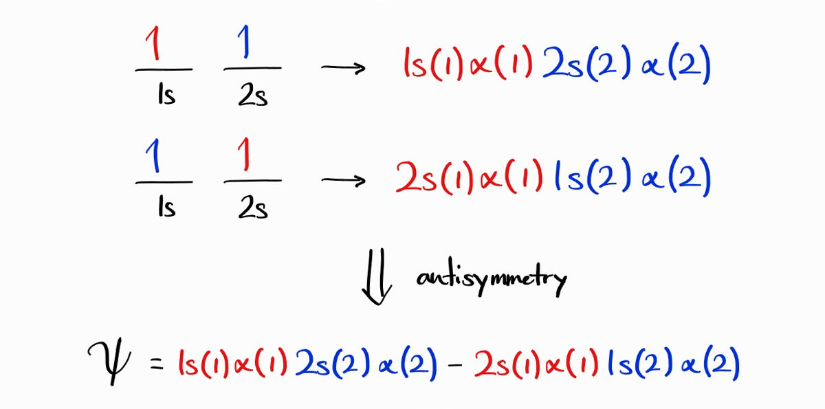
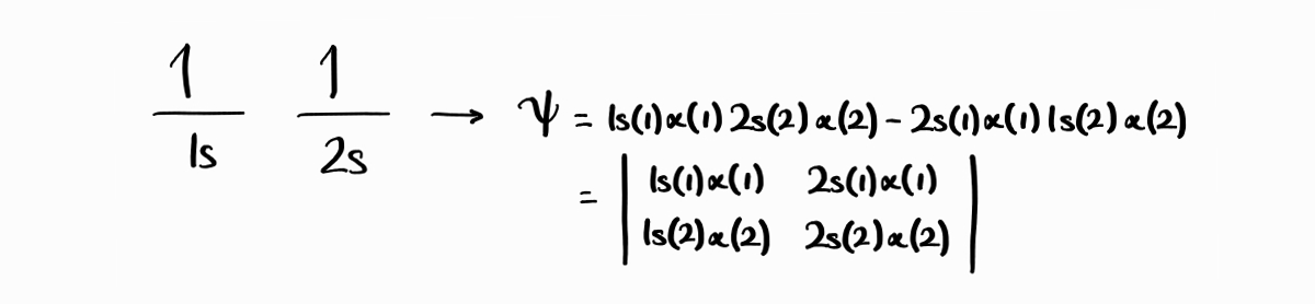
Are these two wave functions, $1s(1)\alpha(1)\,2s(2)\alpha(2)$ and $2s(1)\alpha(1)\,1s(2)\alpha(2)$, valid electronic wave functions? The answer is no as they are not antisymmetric. However, the exchange of two electrons rather results in the wave function taking the form of the other wave function. Taking inspiration from this strange property, we can make a new wave function that is antisymmetric from the linear combination of the two: $1s(1)\alpha(1)2s(2)\,\alpha(2)-2s(1)\alpha(1)\,1s(2)\alpha(2)$. Note that Slater determinants can be used to set up antisymmetric wavefunctions with ease.

The wave function for the second microstate, with both electrons spin down, can be made by changing both electrons to be spin down: $1s(1)\beta(1)\,2s(2)\beta(2)-2s(1)\beta(1)\,1s(2)\beta(2)$.

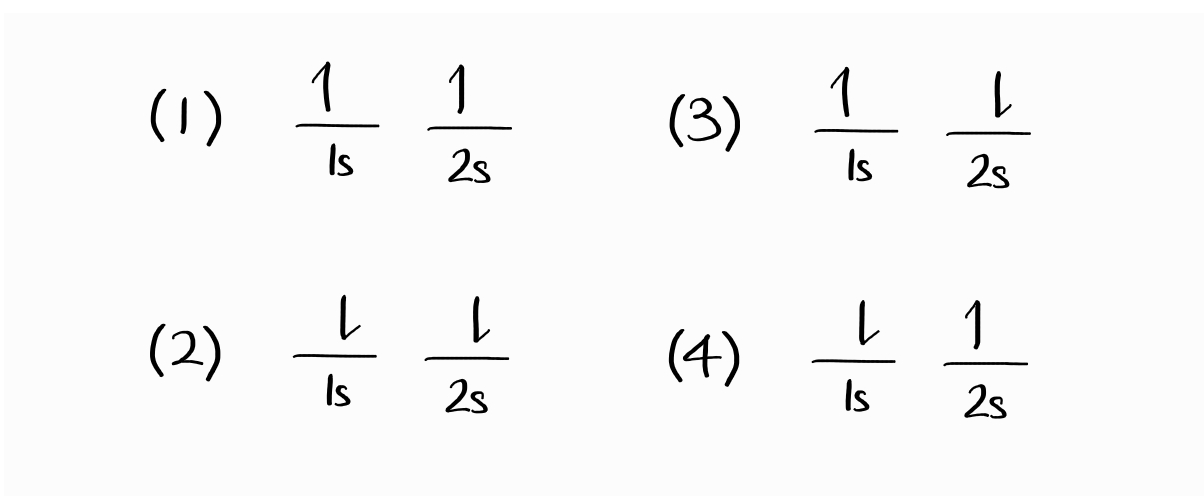
The third and fourth microstate are a bit different. The third microstate, with the $1s$ electron spin up and the $2s$ electron spin down, results in two plausible wave functions: $1s(1)\alpha(1)\,2s(2)\beta(2)$ and $2s(1)\beta(1)\,1s(2)\alpha(2)$. The fourth microstate, with the $1s$ electron spin down and the $2s$ electron spin up, results in $1s(1)\beta(1)\,2s(2)\alpha(2)$ and $2s(1)\alpha(1)\,1s(2)\beta(2)$.

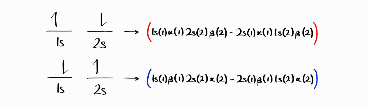
You might assume that the third microstate produces the wave function $1s(1)\alpha(1)\,2s(2)\beta(2) - 2s(1)\beta(1)\,1s(2)\alpha(2)$, and the fourth microstate produces the wave function $1s(1)\beta(1)\,2s(2)\alpha(2)-2s(1)\alpha(1)\,1s(2)\beta(2)$, both of which are suitable antisymmetric wave functions. This is not the case for two major reasons.

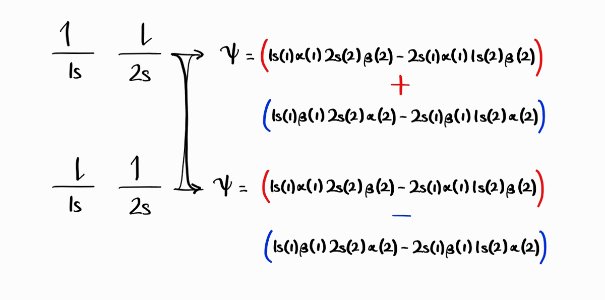
The first reason is the indistinguishable nature of electrons. We have seen that the $1s$ electron of the third microstate is spin up, and the $1s$ electron of the fourth microstate is spin down. However, for any energy state, any electron must be spin up or down with the same probability. Thus, for any energy state, the $1s$ electron is a 1:1 linear combination of spin up and spin down state (this is true for the $2s$ electron). Switching our perspective from spin to orbitals, for any energy state, any electron must be in the $1s$ orbital or the $2s$ orbital with the same probability. Thus, for any energy state, the spin up electron is a 1:1 linear combination of $1s$ and $2s$ orbital state (this is also true for the spin down electron). To conclude, linear combinations of the two antisymmetric wave functions must be taken to produce the adequate wave functions for the third and fourth energy state. Addition produces one wave function (still antisymmetric) that describes the one of the energy states, while subtraction produces the wave function (antisymmetric as well) of the other energy state.

Therefore, $1s(1)\alpha(1)\,2s(2)\beta(2) - 2s(1)\beta(1)\,1s(2)\alpha(2) + 1s(1)\beta(1)\,2s(2)\alpha(2) - 2s(1)\alpha(1)\,1s(2)\beta(2)$ and $1s(1)\alpha(1)\,2s(2)\beta(2) + 2s(1)\beta(1)\,1s(2)\alpha(2) - 1s(1)\beta(1)\,2s(2)\alpha(2) - 2s(1)\alpha(1)\,1s(2)\beta(2)$ are our wave functions for the third and fourth energy states.

The second reason (which is a consequence of the first reason) is that the two new antisymmetric wave functions are eigenfunctions of $\hat{H}, \hat{L}^2, \hat{L}_z, \hat{S}^2, \hat{S}_z$, while the two old antisymmetric wave function were not.

To conclude, we have constructed four wave functions from four microstates for $1s^12s^1$, as follows. These four wave functions are chosen such that they are eigenfunctions of $\hat{H}, \hat{L}^2, \hat{L}_z, \hat{S}^2, \hat{S}_z$ simultaneously. An important point to note is the fact that the number of microstates equals the number of wave functions (energy states).

$$1s(1)\alpha(1)\,2s(2)\alpha(2)-2s(1)\alpha(1)\,1s(2)\alpha(2)$$ $$1s(1)\beta(1)\,2s(2)\beta(2)-2s(1)\beta(1)\,1s(2)\beta(2)$$ $$1s(1)\alpha(1)\,2s(2)\beta(2) - 2s(1)\beta(1)\,1s(2)\alpha(2) + 1s(1)\beta(1)\,2s(2)\alpha(2) - 2s(1)\alpha(1)\,1s(2)\beta(2)$$ $$1s(1)\alpha(1)\,2s(2)\beta(2) - 2s(1)\beta(1)\,1s(2)\alpha(2) - 1s(1)\beta(1)\,2s(2)\alpha(2) + 2s(1)\alpha(1)\,1s(2)\beta(2)$$

In determinantal form (recall Slater determinants)²:

$$\begin{vmatrix} 1s(1)\alpha(1) & 2s(1)\alpha(1)\\ 1s(2)\alpha(2) & 2s(2)\alpha(2) \end{vmatrix}$$ $$\begin{vmatrix} 1s(1)\beta(1) & 2s(1)\beta(1)\\ 1s(2)\beta(2) & 2s(2)\beta(2) \end{vmatrix}$$ $$\begin{vmatrix} 1s(1)\alpha(1) & 2s(1)\beta(1)\\ 1s(2)\alpha(2) & 2s(2)\beta(2) \end{vmatrix} + \begin{vmatrix} 1s(1)\beta(1) & 2s(1)\alpha(1)\\ 1s(2)\beta(2) & 2s(2)\alpha(2) \end{vmatrix}$$ $$\begin{vmatrix} 1s(1)\alpha(1) & 2s(1)\beta(1)\\ 1s(2)\alpha(2) & 2s(2)\beta(2) \end{vmatrix} - \begin{vmatrix} 1s(1)\beta(1) & 2s(1)\alpha(1)\\ 1s(2)\beta(2) & 2s(2)\alpha(2) \end{vmatrix}$$

For two-electron systems, the spatial part and the spin part can be factored out. This factored form is useful when seeing how they are antisymmetric, as well as when calculating various properties.

$$\left[1s(1)\,2s(2)-2s(1)\,1s(2)\right]\alpha(1)\alpha(2)$$ $$\left[1s(1)\,2s(2)-2s(1)\,1s(2)\right]\beta(1)\beta(2)$$ $$\left[1s(1)\,2s(2) - 2s(1)\,1s(2)\right]\left[\alpha(1)\,\beta(2) + \beta(1)\,\alpha(2)\right]$$ $$\left[1s(1)\,2s(2) + 2s(1)\,1s(2)\right]\left[\alpha(1)\,\beta(2) - \beta(1)\,\alpha(2)\right]$$

We can directly apply the operators $\hat{L} ^2 = \left(\hat{l} _1 + \hat{l} _2\right) ^2$, $\hat{L}_z = \hat{l} _{1z} + \hat{l} _{2z}$, $\hat{S} ^2 = \left(\hat{s} _1 + \hat{s} _2\right) ^2$, and $\hat{S} _z = \hat{s} _{1z} + \hat{s} _{2z}$ to the wave functions above to obtain $\left|\bold{L}\right| ^2, L_z \left|\bold{S}\right| ^2,$ and $S_z$ and therefore $L, M_L, S,$ and $M_S$. For example, with the spin part of the first wave function,

$$\hat{S}_z \left(\alpha(1)\alpha(2)\right) = \left(\hat{s}_{1z} + \hat{s}_{2z}\right)\alpha(1)\alpha(2)$$ $$= \hat{s}_{1z}\,\alpha(1)\alpha(2) + \alpha(1)\,\hat{s}_{2z}\,\alpha(2)$$ $$= \left(+\frac{1}{2}\hbar\right)\alpha(1)\,\alpha(2) + \alpha(1)\left(+\frac{1}{2}\hbar\right)\alpha(2)$$ $$= +\hbar \left(\alpha(1)\alpha(2)\right)$$

Therefore, $S_z = +\hbar$ and $M_S = +1$. Calculating $M_L$ and $M_S$ for all four wave functions is a good exercise in manipulating operators.

These are the results:

Spatial part	$L$	$M_L$	Spin part	$S$	$M_S$	Term Symbol
$1s(1)\,2s(2)-2s(1)\,1s(2)$	0	0	$\alpha(1)\alpha(2)$	1	+1	$^3S$
$1s(1)\,2s(2)-2s(1)\,1s(2)$	0	0	$\beta(1)\beta(2)$	1	-1	$^3S$
$1s(1)\,2s(2)-2s(1)\,1s(2)$	0	0	$\alpha(1)\,\beta(2) + \beta(1)\,\alpha(2)$	1	0	$^3S$
$1s(1)\,2s(2)+2s(1)\,1s(2)$	0	0	$\alpha(1)\,\beta(2) - \beta(1)\,\alpha(2)$	0	0	$^1S$

From the possible $L$ and $S$ values, we can see that the term symbols that describe $1s^12s^1$ are $^3S$ (triply degenerate) and $^1S$ (singly degenerate).

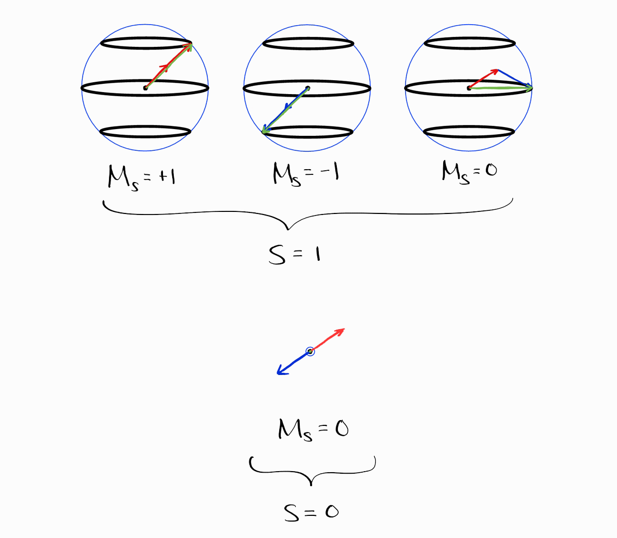
On a side note, the spin parts can be added in a visual way (ignoring the spatial parts). The following are representations of spin functions $\alpha$ and $\beta$.

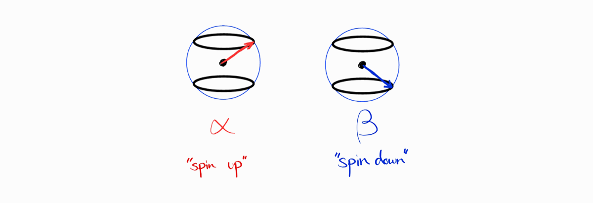
These spin functions are multiplied and added to produce the spin parts, shown in the table above.

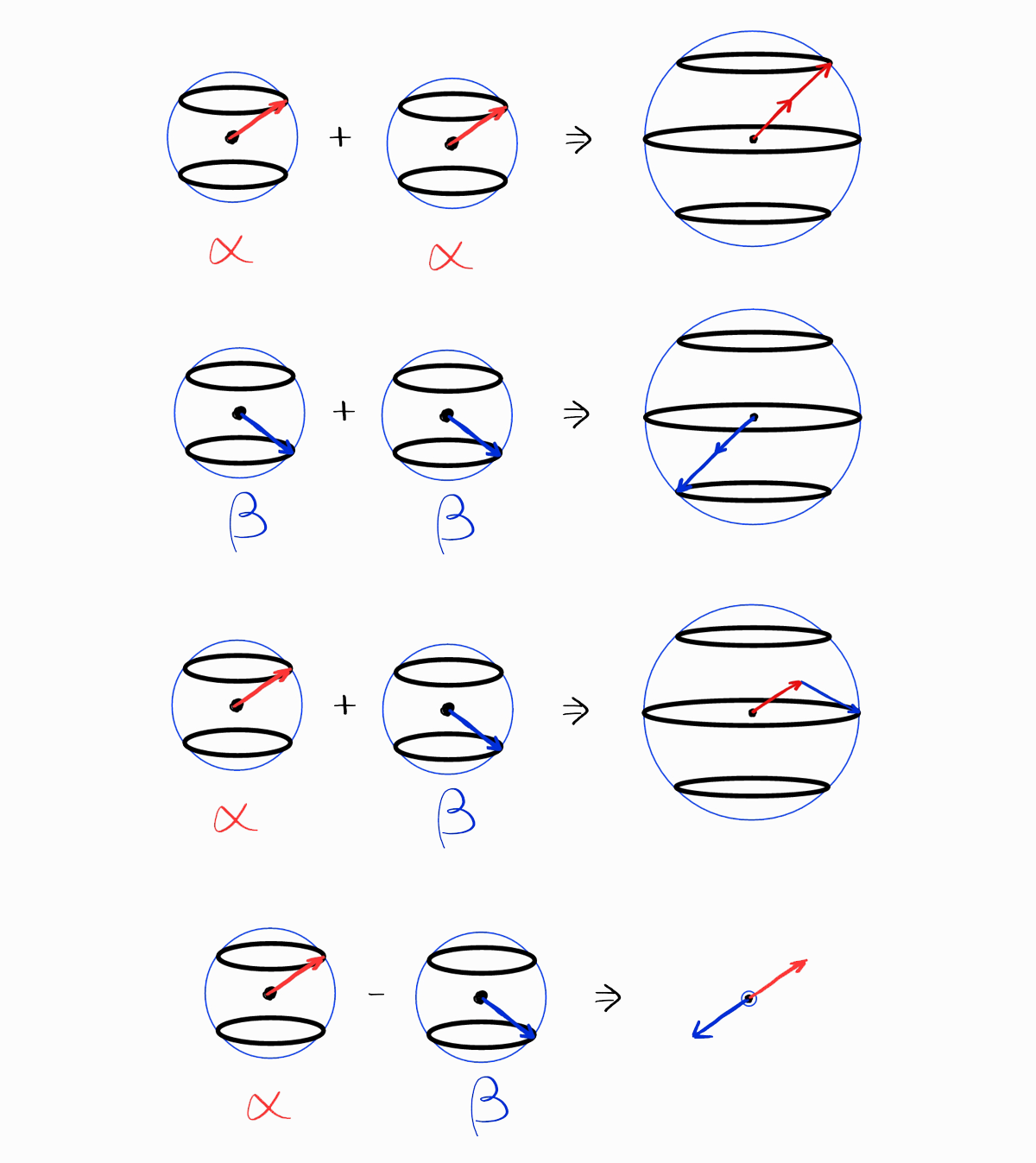
The resulting visual representations clearly show the $S$ and the $M_S$ of the spin functions, which is the same as the table above.

Coming back to our results of approach 1, the shortcomings of this approach is that you first need to obtain each and every wave function before anything else. Is there a way to obtain the term symbols without the wave functions?

Approach 2: $M_L$ and $M_S$ from microstates

In the procedure above, calculating $M_L$ and $M_S$ from wave functions is easy. What is easier is calculating $M_L$ and $M_S$ from the four original microstates.

Recall that $\hat{S} _z = \hat{s} _{1z} + \hat{s} _{2z}$. For the appropiate eigenfunctions (which is the case for all examples in this section), $S _z = s _{1z} + s _{2z}$ and thus, for the quantum number $M _S = m _{s1} + m _{s2}$.

The first microstate has both electrons spin up. Therefore, $M_S = +\frac{1}{2}:+\frac{1}{2} = +1$. The second microstate has both electrons spin down, so $M_S = -\frac{1}{2}:-\frac{1}{2} = -1$. The third and fourth microstates has one electron spin down and another spin up, which results in $M_S = 0$.

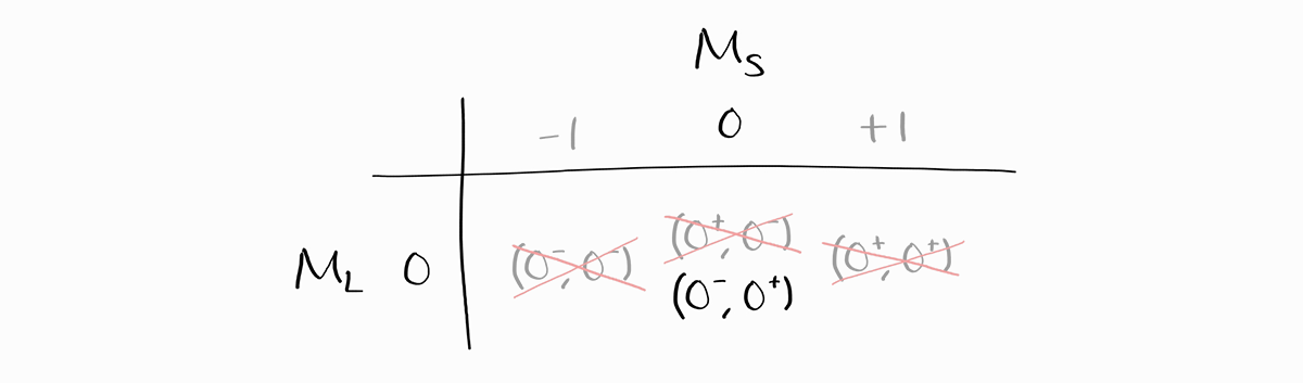
For all four microstates, $M_L = 0$ as $m_l$ for both $1s$ and $2s$ orbitals are 0. We can organize these microstates into a table. They are given as $\left( 0^+, 0^- \right)$, which means $m_{l1} = 0, m_{s1} = +1/2, m_{l2} = 0,$ and $m_{s2} = -1/2$.

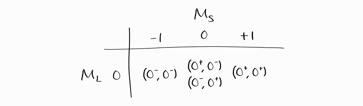
Now, we will obtain the term symbols by progressively erasing the (micro)states of each term symbol.

From these values of $M_L$ and $M_S$, note that the maximum value of $M_S$ is +1 and the minimum value is -1. Assume for a moment that $S$ of a term symbol is larger than 1. Then, the maximum value of $M_S$ should be larger than +1, and the minimum value of $M_S$ should be smaller than -1. As that is not the case, $S$ is not larger than 1, and as a consequence, the largest $S$ possible a term symbol can have must be 1.

As the maximum value of $M_L$ is 0, it must be that $L = 0$. Thus, the largest possible combination of $S$ and $L$ is $L = 0$ and $S = 1$. This is $^3S$ in term symbol notation, which consists of three states: $M_L = 0$ and $M_S = -1, \,0, \,+1$. After confirming the term symbol $^3S$, we erase three states from the table: one from each possible $M_L$ and $M_S$ to find other term symbols with smaller $S$ and $L$.

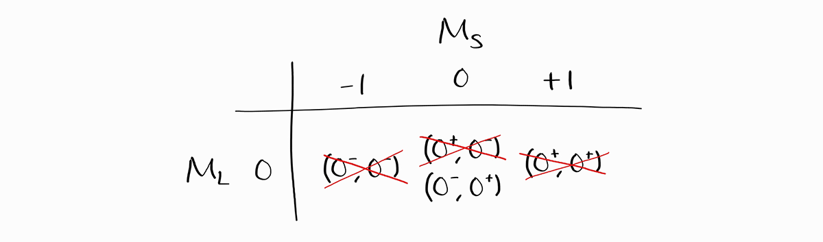
For the entries in $M_L = 0$ and $M_S = 0$, the microstate $\left(0^+, 0^-\right)$ is erased instead of $\left(0^-, 0^+\right)$. This does not mean that $^3S$ contains the microstate $\left(0^+, 0^-\right)$ but not $\left(0^-, 0^+\right)$; it merely means that one of two states with $M_L = 0$ and $M_S = 0$ is in $^3S$, while the term symbol for the other state is yet to be determined. The most technically accurate way to erase these states would be erase one-half of both states, but that can result in confusion. Instead, a single state (either one) is completely erased for visual clarity, and the choice of microstate to be erased is unimportant.

Now, the maximum value of $M_S$ is 0, and the maximum value of $M_L$ is 0. Thus, the only possible combination of $L$ and $S$ is $L = 0$ and $S = 0$, resulting in a term symbol of $^1S$. We cross out the microstate in $L = 0$ and $S = 0$, which leaves us with no remaining states. All term symbols of $1s^12s^1$ have been accounted for.

Quantum Mechanical Addition of Angular Momenta

Although approach 2 is a lot quicker than approach 1, there is yet a faster way to obtain the term symbols of $1s^12s^1$ by generalizing approach 2. Recall how the sum of the largest values of $m_{s1} (+\frac{1}{2})$ and $m_{s2} (+\frac{1}{2})$ adds to give the largest value of $M_S (+1)$. This is equal to the sum of $s_1 \left(\frac{1}{2}\right)$ and $s_2 \left(\frac{1}{2}\right)$, as the largest value of $m_{s1}$ is $s_1$ and the largest value of $m_{s2}$ is $s_2$.

Now consider an addition of a general angular momentum quantum numbers $j_1$ and $m_{j1}$ with $j_2$ and $m_{j2}$, resulting in $J$ and $M_J$ (alongside $j_1$ and $j_2$, which are implicitly understood) (the image below has $j_1 = \frac{3}{2}$ and $j_2 = 1$).

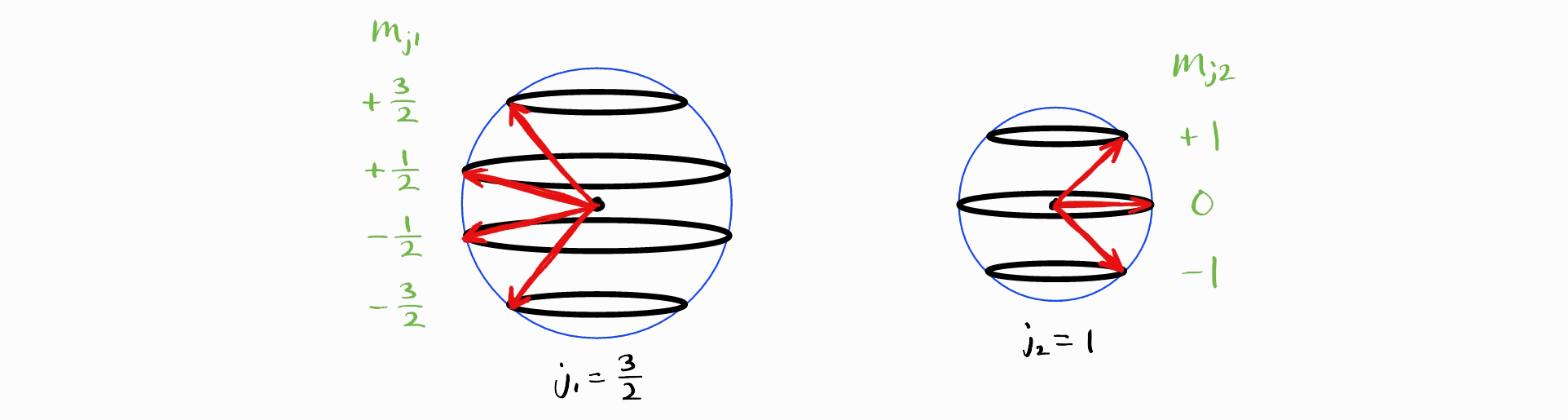
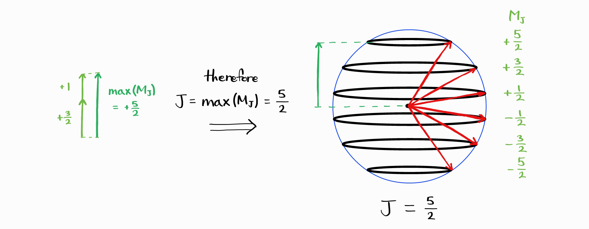
The largest value of $M_J$ is $j_1+j_2$.

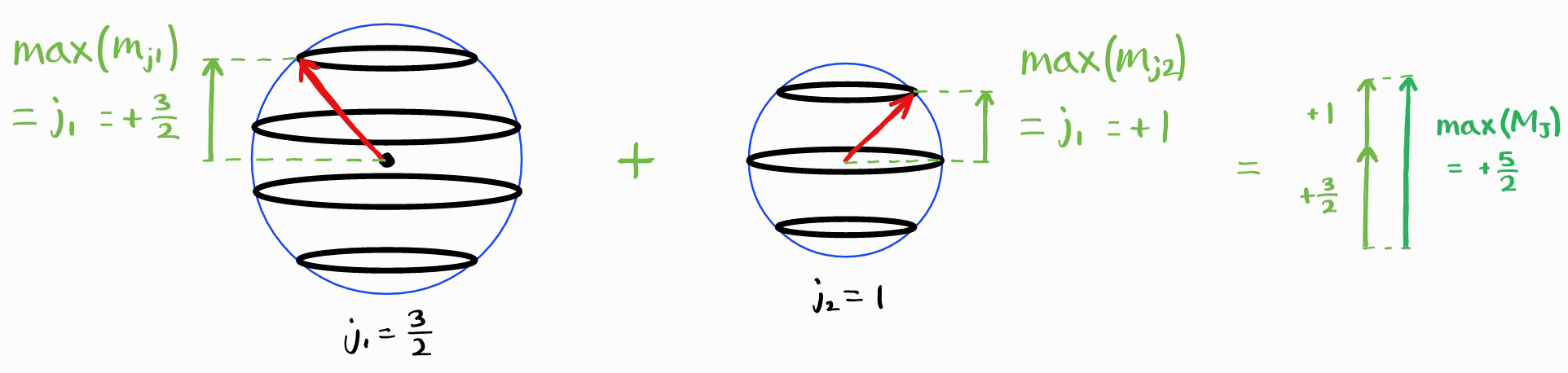
The largest possible $J$ is therefore $j_1+j_2$. Like all angular momentum quantum numbers, $M_J$ can have the values $+J, \,+J-1,\,\cdots,\, -J+1, -J$.

If $J_{\text{max}} = j_1 + j_2$, then what is $J_{\text{min}}$? The smallest maximum value of $M_J$ is given by the difference of the largest values of $m_{j1}$ and $m_{j2}$. This is equal to the difference between $j_1$ and $j_2$.

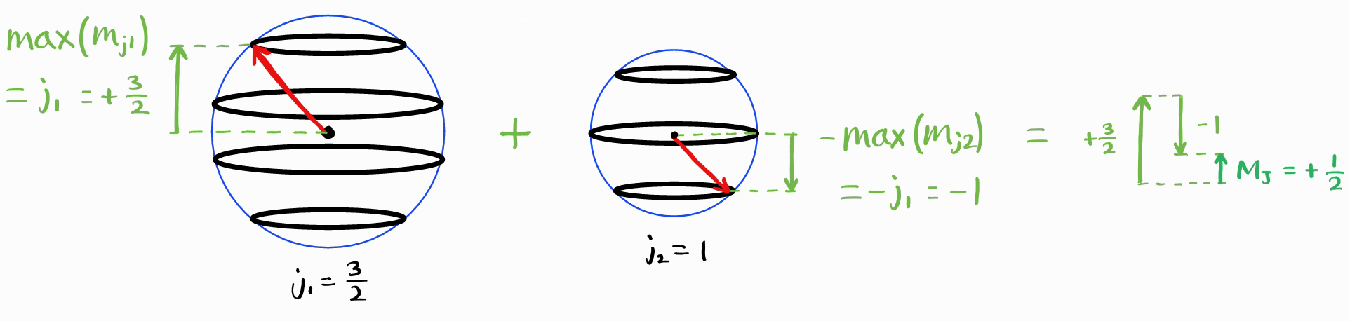
Thus, the smallest maximum value of $M_J$ is $\left|j_1 - j_2\right|$. Therefore, smallest possible $J$ is $\left|j_1 - j_2\right|$.

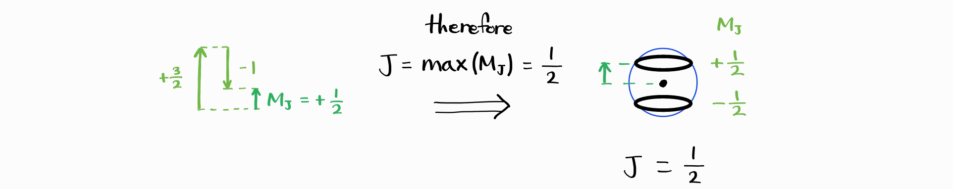
Therefore, $J_{\text{min}} = \left|j_1 - j_2\right|$. Thus, the possible $J$ are $\left|j_1 - j_2\right|,\,\cdots,\,j_1 + j_2$. Just as a check, let us compare the total number of microstates (total number of combinations of $j_1$, $m_{j1}$, $j_2$, $m_{j2}$), with the total number of states (total number of combinations of $j_1$, $j_2$, $J$ and $M_J$). As $j_1$ and $j_2$ are fixed, the former is equal to $\left(2j_1+1\right)\left(2j_2+1\right)$. The latter is equal to $\sum_J \left(2J+1\right)$, summed over $J = \left|j_1 - j_2\right|,\,\cdots,\,j_1 + j_2$.

$$\left(2j_1+1\right)\left(2j_2+1\right) = \sum_{J\,=\,\left|j_1 - j_2\right|}^{j_1 + j_2} \left(2J+1\right)$$

With some algebraic manipulation, this can be shown to be true. We are left with a general statement on the addition of angular momenta.

The addition of two angular momenta characterized by quantum numbers $j_1$ and $j_2$ results in a total angular momentum whose quantum number $J$ has the possible values

$$J=\left|j_1 - j_2\right|,\,\left|j_1 - j_2\right|+1,\,\cdots,\,j_1 + j_2 - 1,\,j_1 + j_2$$

Approach 3: direct addition

Let us apply this for the $L$ and $S$ of $1s^12s^1$. For the electron in the $1s$ orbital, $l_1 = 0$ ($s$ orbital). For the electron in the $2s$ orbital, $l_2 = 0$. Therefore, $L_{\text{min}} = \left| 0 - 0 \right| = 0$ and $L_{\text{max}} = 0 + 0 = 0$. This means that $L = 0$.

As for spin, both electrons have $s = 1/2$. $S_{\text{min}} = \left| 1/2 - 1/2 \right| = 0$ and $S_{\text{max}} = 1/2 + 1/2 = 1$. Therefore, $S = 0, 1$.

Combining both $L = 0$ and $S = 0, 1$ result in the term symbols $^1S$ and $^3S$. Notice how simple this approach is - how there was no need to fumble around with $M_L$ and $M_S$.

There is one critical caveat to this approach; it cannot be used with equivalent electrons, which are electrons in the same subshell. For example, the steps above, when applied to $1s^2$, should result in the same term symbols. However, due to the Pauli exclusion principle, the two electrons cannot have parallel spins and $S = 1$ is impossible. Instead, the two electrons have opposite spins, and only $M_S = 0$ is allowed. Thus, the only term symbol possible for $1s^2$ is $^1S$.

As a simple exercise, let us tackle $1s^12s^13s^1$. For this configuration, we split it into $1s^12s^1$ and $3s^1$. We know the $l_1$ & $s_1$ of $1s^12s^1$ - it is the same as our previous answer: $l_1 = 0$ & $s_1 = 0, 1$. For $3s^1$, $l_2 = 0$ ($s$ orbital) & $s_2 = 1/2$.

There are two additions possible: (1) between $l_1 = 0$ & $s_1 = 0$ and $l_2 = 0$ & $s_2 = 1/2$, or (2) between $l_1 = 0$ & $s_1 = 1$ and $l_2 = 0$ & $s_2 = 1/2$.

For (1), $l_1 = 0$ adds with $l_2 = 0$ to produce $L_{\text{min}} = \left|0 - 0\right| = 0$ and $L_{\text{max}} = 0 + 0 = 0$, resulting in $L = 0$. This is unsurprising as all electrons are in an $s$ orbital. $s_1 = 0$ and $s_2 = 1/2$ results in $S_{\text{min}} = \left|0 - \frac{1}{2}\right| = \frac{1}{2}$ and $S_{\text{max}} = 0 + \frac{1}{2} = \frac{1}{2}$. Therefore, $L = 0$ and $S = 1/2$, and the term symbol is $^2S$.

For (2), $l_1 = 0$ adds with $l_2 = 0$ to produce $L = 0$; same as before. $s_1 = 1$ and $s_2 = 1/2$ results in $S_{\text{min}} = \left|1 - \frac{1}{2}\right| = \frac{1}{2}$ and $S_{\text{max}} = 1 + \frac{1}{2} = \frac{3}{2}$. Therefore, $L = 0$ and $S = 1/2,\, 3/2$, and the term symbols are $^2S$ and $^4S$.

In conclusion, $1s^12s^13s^1$ results in the term symbols $^2S$ (two) and $^4S$.

Spin-Orbit Coupling

Remember this?

The energy level of an atom is characterized by the electron configuration, the total orbital angular momentum quantum number $L$, and the total spin quantum number $S$.

I lied. It turns out that a quantum mechanical effect called spin-orbit interaction (or spin-orbit coupling) effects the energy of the energy state ever so slightly. The energy states with the same electron configuration, $L$, and $S$ are nearly degenerate, but not completely degenerate. For an explanation on this effect, we must return to the Hamiltonian $\hat{H}$.

In part 1, the following was the multi-electron $\hat{H}$ in atomic units.

$$\hat{H} = \hat{H}^{(0)} = \sum_{i\,=\,1}^{n}\left ( -\frac{1}{2}\nabla_i^2 \right ) + \sum_{i\,=\,1}^{n}\left ( -\frac{Z}{r_i} \right ) + \sum_{i}\sum_{j\,>\,i} \left ( \frac{1}{r_{ij}} \right )$$

With this Hamiltonian (denoted $\hat{H}^{(0)}$), the operators $\hat{L}^2$, $\hat{L}_z$, $\hat{S}^2$, and $\hat{S}_z$ all commute with $\hat{H}^{(0)}$, which results in the energy states with the same electron configuration, $L$, and $S$ being degenerate. However, the true Hamiltonian, $\hat{H}$, contains a term ($\hat{H}^{(1)}$) that is dependent on $\hat{\bold{l}}_i\cdot\hat{\bold{s}}_i$ for all electrons in an atom. Roughly speaking, the term $\hat{\bold{l}}_i\cdot\hat{\bold{s}}_i$ represents the interaction between the magnetic moment due to the electron spin with the magnetic field generated by the electron’s orbit. The true Hamiltonian is thus closer to the following (the function $\xi(r_j)$ is not important for our discussion).

$$\hat{H} = \hat{H}^{(0)} + \hat{H}^{(1)} = \sum_{i\,=\,1}^{n}\left ( -\frac{1}{2}\nabla_i^2 \right ) + \sum_{i\,=\,1}^{n}\left ( -\frac{Z}{r_i} \right ) + \sum_{i}\sum_{j\,>\,i} \left ( \frac{1}{r_{ij}} \right ) + \sum_{i\,=\,1}^{n} \left( \xi(r_i)\, \hat{\bold{l}}_i\cdot\hat{\bold{s}}_i \right)$$

Note that for elements with atomic number less than 30, the effect of $\hat{H}^{(1)}$ is much smaller than $\hat{H}^{(0)}$. As a result, $\hat{L}^2$, $\hat{L}_z$, $\hat{S}^2$, and $\hat{S}_z$ nearly commutes with $\hat{H}$, and a microscopic energy difference of

$$E^{(1)} \approx \frac{1}{2}A[J(J+1) - L(L+1) - S(S+1)]$$

can be seen for multi-electron atoms. This difference of 0.1% breaks the degeneracy previously seen with $L$ and $S$.⁴

If so, what is $J$ from the equation above? For starters, $\bold{J}$ is the total angular momentum, which is equal to $\bold{L} + \bold{S}$. This coupling between total orbital angular momentum $\bold{L}$ and total spin angular momentum $\bold{S}$ is called L-S coupling or Russell-Saunders coupling. In operator form,

$$\hat{J} = \hat{L} + \hat{S}$$

Just like $\hat{L}$ and $\hat{S}$, $\hat{J}$ has its own quantum numbers ($J$ and $M_J$) which satisfy the following relations (note that $M_J = -J, \,-J+1,\,\cdots,\,+J-1,\,+J$).

$$\hat{J}^2 \psi = \left\| \bold{J} \right\|^2 \psi =J\left(J+1\right)\hbar^2 \psi$$ $$\hat{J}_z \psi = J_z \psi = M_J \hbar \, \psi$$

Previously, $\hat{H}$, $\hat{L}^2$, $\hat{L}_z$, $\hat{S}^2$, and $\hat{S}_z$ commuted with each other to form a complete set of commuting observables. Now, $\hat{H}$, $\hat{L}^2$, $\hat{S}^2$, $\hat{J}^2$, and $\hat{J}_z$ commute to form a complete set of commuting observables.

Therefore, $L$, $S$, $J$, and $M_J$ are used to specify an energy state instead of $L$, $M_L$, $S$, and $M_S$. To specify an energy level (term symbol), $L$, $S$, and $J$ are required. $M_J$ is excluded as states with different $M_J$ but same $L$, $S$, and $J$ are degenerate as $M_J$ is not included in $E^{(1)}$.

If so, what is the value of $J$ for a given $L$ and $S$? Just like adding two orbital angular momentum quantum numbers $l_1$ and $l_2$ or two spin quantum numbers $s_1$ and $s_2$, we can obtain $J$, the total angular momentum quantum number by “adding” $L$ and $S$.

For $L$ and $S$, the possible values of $J$, the total angular momentum quantum number, are

$$J=\left|L - S\right|,\,\left|L - S\right|+1,\,\cdots,\,L + S - 1,\,L + S$$

For example, $L = 1$ and $S = 1$. The possible values of $J = 0, 1, 2$.

As $L$, $S$, and $J$ are all required to specify an energy level, the term symbol notation changes from $^{2S+1}L$ to¹

$$^{2S+1}L_J$$

The degeneracy of this term symbol is now $2J+1$ (the total number of possible $M_J$), instead of $\left(2L+1\right)\left(2S+1\right)$.

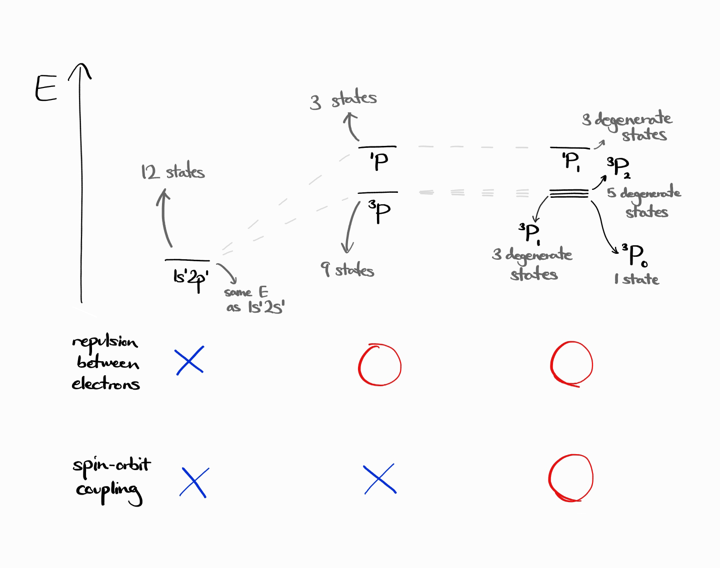
For $L = 1$, $S = 1$, as $J = 0, 1, 2$, the new term symbols are $^3P_0, ^3P_1$, and $^3P_2$ instead of just $^3P$. In other words, the 9 degenerate $^3P$ energy states are actually 1 state belonging to $^3P_0$, 3 degenerate states belonging to $^3P_1$, and 5 degenerate states belonging to $^3P_2$. As demonstrated, the number of states do not change. For a given $L$ and $S$,

$$\left(2L+1\right)\left(2S+1\right) = \sum_{J \, = \, \left| L - S \right|}^{L+S}\left(2J+1\right)$$

Conclusion

Here is a quick recap of all the things we learned about term symbols.

1. The energy of an energy state is determined by its electron configuration and its quantum numbers: the total orbital angular momentum quantum number $L$, the total spin quantum number $S$, and the total angular momentum quantum number $J$.
2. To describe an energy level, we use atomic term symbols: $^{2S+1}L_J$

To obtain the term symbol for a particular electron configuration, there are two practical options, which are approaches 2 and 3:

Approach 3: for non-equivalent electrons only

• Perform addition of angular momenta to obtain $L$ and $S$
• Perform addition of $L$ and $S$ to obtain $J$

Approach 2: for equivalent electrons⁵

• Organize all microstates into a table according to their $M_L$ and $M_S$, then progressively erase microstates that belong to a term symbol with the largest possible $L$ and $S$
• Obtain $J$ for all term symbols through addition of $L$ and $S$

As a quick problem, try to find the term symbols of $1s^12p^1$ excited state helium by yourself!

















The term symbols are $^3P_0$, $^3P_1$, $^3P_2$, and $^1P_1$. The following is an energy diagram of those term symbols, which also shows how the energy and degeneracies of energy level changes due to the change in Hamiltonian.

Footnotes

1. In some textbooks (such as Levine), a term refers to an “energy level” (determined by electron configuration, $L$, and $S$, but not $J$), while a term symbol refers to the symbol that is used to represent the term. In this case, term is a closely spaced set of energy levels (which are determined by electron configuration, $L$, $S$, and $J$). ↩ ↩²

2. If you are unfamiliar with this notation, see page 284 of McQuarrie. Note that all wave functions dealt in this article are not normalized but are normalizable. ↩ ↩²

3. Electron configuration like this are called microstates because it treats each electron as independent, as if the quantum number (thus the state) of each electron is obtainable. The states of each electron is thought to combine to form the entire atom, which is considered as a macrostate. ↩

4. This results in the fine structure of atomic spectra. ↩

5. Also possible for non-equivalent electrons. ↩